Tools

8. Tools

Search (Ctrl+K)

Tools > Search or press Ctrl+K / Cmd+K.

Opens a search dialog for quickly locating any device or interface. Type to search across:

• Router ID, Hostname, DNS Name, Label, Vendor (device fields)
• Interface name, IP address, interface description (interface fields)
• CIDR subnet containment (e.g., entering 192.168.1.0/24 finds all interfaces in that subnet)

Results are grouped into Devices and Interfaces sections with match highlighting. Use arrow keys to navigate results, Enter to select. The selected device is highlighted on the canvas and its Node Detail Panel opens.

Time Travel

Tools > Time Travel, or click the clock button in the bottom bar's mode cluster.

View the network topology at any historical point:

1. Activate Time Travel to show the time scrubber bar at the bottom of the screen.
2. The bar has transport controls: skip backward/forward, step, play/pause.
3. Adjust playback speed (0.5x to 10x) and the time window (1h–30d or a custom range).
4. Drag the scrubber slider to any point in time.
5. The topology canvas reconstructs the historical state from snapshots.
6. A blue tint and TIME TRAVEL label on the bar indicate you're viewing historical data (amber = simulation).
7. Click the green Go Live button to return to real-time.

Keyboard shortcuts while in Time Travel mode: Space (play/pause), Left arrow (step backward), Right arrow (step forward).

Time travel uses hash-deduplicated per-area JSONB snapshots, so only actual changes consume storage.

When time travel is active, the Node Detail Panel and Link Detail Panel adapt automatically:

• An amber banner shows "Viewing at [timestamp]" at the top.
• Critical state banners (device down / link down) reflect the historical topology state at the playback timestamp.
• Live traffic polling and boost are suppressed.
• The Events section filters to ±1 hour around the playback timestamp.
• Utilization charts show a vertical highlight marker at the playback time.

What time travel does not reconstruct. A few things have no history, and the product shows their absence instead of dressing live data as historical:

• Utilization coloring switches off. View > Color > By Utilization drops its colors at a historical time — the canvas deliberately does not paint today's traffic onto yesterday's topology. Blank means not available at this time, not no traffic. Per-link utilization history is still available in the Link Detail Panel's charts, with the playback marker.
• LSA header metadata stays live. The LSDB browser reconstructs LSAs and routes as of the selected time, but age/sequence/checksum have no history; a banner in the browser says they keep live values.
• Some path evidence is live. A stitched multi-domain path at a historical time rebuilds its chain from recorded session and RIB history, and names any evidence that is not historized (L2/port annotations, router-id-resolved entries) as explanation steps — see Multi-Domain Paths.
• Per-peer BGP detail needs full recording. Peer-failure assessment, hot-potato analysis and per-peer path expansion at a historical time gate on a BMP target having recorded full history for the scope; without it they state the missing recording instead of approximating.

Combined with Simulation: Time Travel and Simulation can be used simultaneously. Activate time-travel from within simulation (clock icon in the simulation bar) or enter simulation from within time-travel (gear icon in the time-travel bar) — both entries sit next to the Go Live button, and your playback position carries over in both directions (entering simulation keeps the timeline where you were; exiting simulation returns the solo time-travel bar to the same position). Both modes then merge into a single combined bar: an amber SIMULATION + blue TIME TRAVEL context ribbon above the playback controls. Advancing through snapshots during playback automatically re-evaluates SPF with the current mutations applied to each historical snapshot (debounced at 500ms for fast playback). The Go Live split-button exits both modes at once; its dropdown offers Exit Time Travel (stay in simulation) and Exit Simulation (stay in time travel).

Refresh DNS

Tools > Refresh DNS (admin or engineer; hidden for other roles)

Forces a full re-resolution of all PTR (reverse DNS) records for device router IDs and interface IP addresses. Use this when:

• DNS records have been updated (renumbering, device replacement)
• New PTR records have been added
• You want to sync DNS names after zone changes

The refresh happens asynchronously -- the engine clears its DNS cache and re-resolves all cached IPs. Results appear within seconds.

Simulation (What-If Engineering)

Tools > Simulation, or click the gear button in the bottom bar's mode cluster (next to the Time Travel clock).

Simulation (formerly called Engineering Mode) lets you model failure scenarios, cost changes, hypothetical links, and shared risk link group (SRLG) failures on the live topology without affecting the real network. All SPF computation happens server-side using RFC 2328-correct multi-area Dijkstra for OSPF (with inter-area routing via backbone ABRs) and ISO 10589-correct multi-level Dijkstra for IS-IS (with inter-level routing via L1/L2 routers) -- no changes are written to the database.

Entering simulation mode:

When activated, the canvas displays an amber overlay border and a "SIMULATION" watermark to clearly distinguish the simulated view from the live topology. The bottom bar is replaced by the amber simulation bar: SIMULATION label, Baseline/Simulated view toggle, Undo/Redo, a Time Travel entry (clock), the loaded scenario name with mutation count and SPF compute time, the system status cluster, and Go Live to exit. Mutations, impact analysis, paths, batch assessment, and scenarios live in the simulation panel (opens automatically).

Tip: Simulation and Time Travel can be used simultaneously. Click the clock icon in the simulation bar to activate time-travel, or enter Simulation while already viewing historical topology. Simulation results automatically recompute as you advance through snapshots during playback.

Simulating failures and cost changes:

• Right-click a link and select Simulate Failure to take the link down in the simulation, or Change Cost... to open the CostChangePopover for inline OSPF cost editing on that edge.
• Right-click a node and select Simulate Node Failure to take the device and all its links down.

BGP peer failure:

• Right-click a device and select Simulate BGP peer failure... to open the peer picker pre-filtered to that device's own BGP sessions, or click B Peer Failure in the Mutations tab action bar to pick from every peer in scope.
• Peers are grouped by AS number with select-all per group, a search box, and impact badges giving an at-a-glance affected-prefix count per peer.
• Select one or more peers to add them as mutations; the simulation treats each as a downed BGP session. The peer list itself is time-travel aware (fetched as of the selected time), but impact badges are live-only and hidden during time travel -- the impact-summary endpoint has no historical mode.
• Include BGP checkbox (next to the peer-failure button): when enabled, simulations also model BGP hot-potato routing and traffic redistribution effects on top of the IGP-only impact.

Hypothetical routers:

• Right-click empty canvas space and select Add Hypothetical Router... to place a synthetic device on the topology.
• Enter a display name (e.g. "new-core-rtr"). The node appears with a dashed cyan border to distinguish it from real devices.
• The hypothetical router has no area membership at creation — it joins areas when you connect hypothetical links to it, matching real OSPF behavior where area membership is determined by interfaces, not the router.
• If you connect a hypothetical router to devices in two or more areas, it is automatically classified as an ABR.
• Right-click a hypothetical router to remove it (all connected hypothetical links are cascade-deleted) or to add links/simulate failures.

Hypothetical links:

• Right-click a node (real or hypothetical) and select Add Hypothetical Link... to create a synthetic link between two devices.
• Click the source device on the canvas, then click the target device.
• Select the OSPF area for the link. If both devices share exactly one common area, it is auto-selected. If they share multiple areas, choose from a dropdown (shows area ID and protocol). If no common area exists, all areas from both devices are offered with a warning that the other device will be added to the selected area.
• Set the OSPF cost (symmetric by default, or set forward/reverse independently).
• Hypothetical links appear as dashed green edges on the canvas and are included in SPF computation.

SRLG (Shared Risk Link Group):

• Right-click a node and select Start SRLG Group... to begin defining a group.
• While the SRLG panel is open, right-click additional nodes or links and select Add to SRLG Group to accumulate members.
• Name the group and click Create SRLG. The group appears as a single mutation in the Mutations tab, but all members fail simultaneously during SPF computation.
• Load Saved SRLG: Click the "Load Saved SRLG" dropdown to populate members from a persistent SRLG group. Saved SRLGs are managed via Admin > Monitoring > SRLG Groups... (network-scoped, stores link memberships in the database). When a saved SRLG is applied, the server expands it to individual link failures automatically.

SRLG Groups (Admin > Monitoring):

Manage persistent SRLG definitions that can be reused across simulation sessions. Open via Admin > Monitoring > SRLG Groups.... Select a network, then create/edit/delete SRLG groups with named link members. Each SRLG is scoped to a single network and stores its member links in the database. These groups appear in the "Load Saved SRLG" dropdown during simulation.

SimulationPanel (right side, 380px):

At the left of the tab bar an instance selector shows which protocol instance the simulation targets (e.g. "OSPFv3 (IPv6) · pid 0"). The canvas can show several routing instances at once, but a simulation always evaluates against a single instance. When more than one instance is visible, click the selector to switch which one the simulation runs against — this re-scopes the active instance, so the simulation, its scenarios and the area clouds all follow it (the simulated scope always matches what you are looking at). Every instance stays drawn — your checked areas don't change; only the simulation and cloud focus move. The saved topology layout is shared across every protocol instance in the routing domain (positions key on router ID), so node positions stay put when you switch instances. Existing mutations are kept and re-evaluated against the newly selected instance (mutations that don't apply to it are ignored). With a single instance in view it is just a label.

The simulation panel has 3 tabs:

Tab	Purpose
Mutations	Lists all simulated changes (failures, cost overrides, hypothetical routers, hypothetical links, SRLG groups). Add, remove, or toggle individual mutations. Undo/Redo support for iterative exploration. SRLG entries show member count. Includes Scenario Manager for saving and loading named mutation sets (see below).
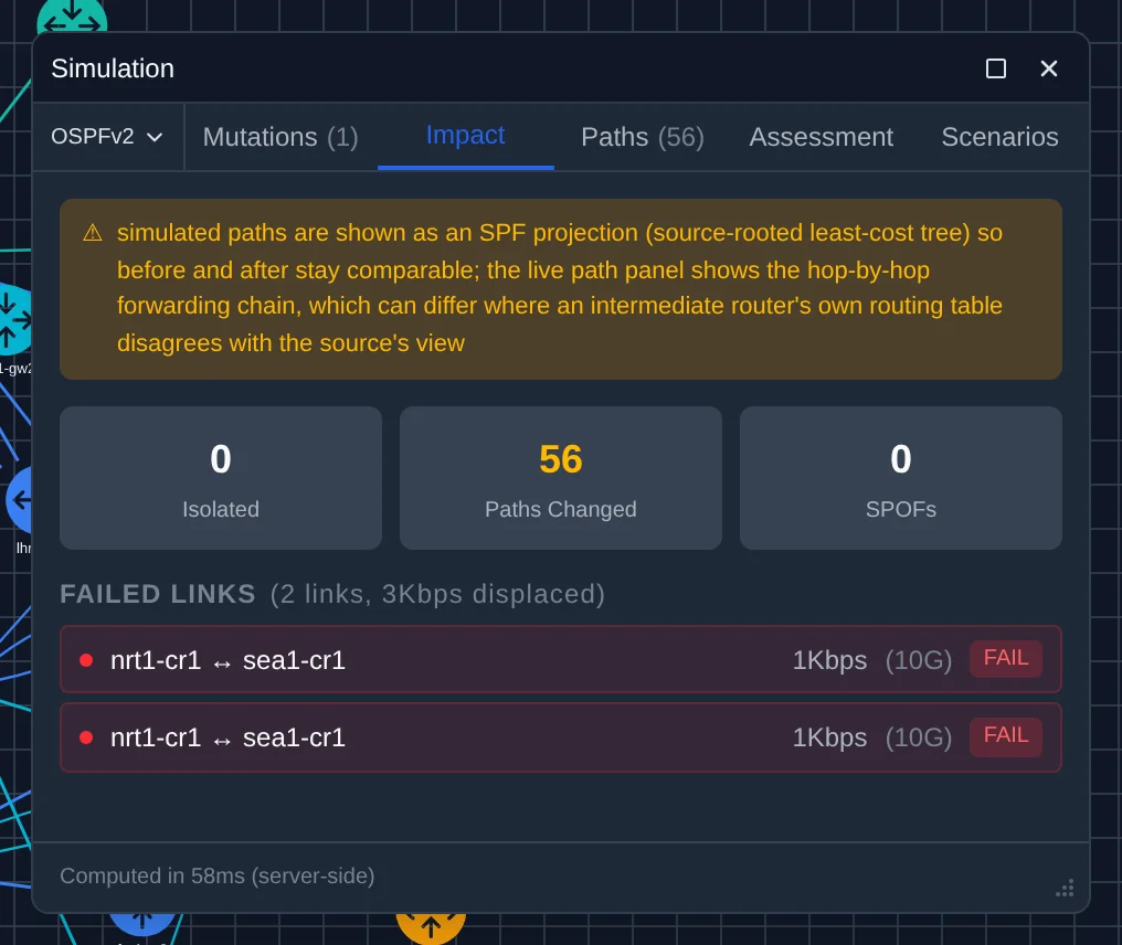
Impact	Shows traffic redistribution: before/after utilization per link, congestion risk badges (ok < 80%, warning 80-95%, critical >= 95%). Also shows isolated devices and affected links.
Paths	Before/after SPF path comparison for all affected device pairs: cost, route type, and hop-by-hop path.

Batch failure assessment:

Open the Assessment tab in the simulation panel to run a batch assessment. This iterates every link or every node in the topology, simulates individual failure for each, and shows which devices become unreachable (isolated from the network).

Only failures that cause actual device isolation are shown — redundant links/nodes whose failure has no isolation impact are filtered out. Click any row to expand it and see the names of the unreachable devices.

Results are displayed in a sortable table. Click column headers to sort by devices lost or entity name. Use Export CSV to download the full assessment for offline analysis.

Scenarios (save/load):

Simulation supports saving mutation sets as named scenarios for reuse, via the Scenarios tab in the simulation panel:

• With mutations active, the tab shows a "Save current mutations" row: type a name and click Save new, or click Update "name" to overwrite the loaded scenario with the current mutations.
• The list below shows all saved scenarios (own + shared). Click any scenario to load its mutations onto the canvas; hover for share/delete actions on your own scenarios.
• Scenarios are stored per-user and scoped to the protocol instance or network.
• Use scenarios to preserve pre-validated maintenance plans, compare alternative failure mitigation strategies, or share standard test cases across sessions.

Workflow example:

1. Click the gear button in the bottom bar (or Tools > Simulation).

2. Right-click a core link and select Simulate Failure.

3. Open the Impact tab to see traffic redistribution and which devices become isolated.

   

4. Open the Paths tab to compare original vs. new path costs for affected device pairs.

5. Right-click another link and select Change Cost... to test a traffic engineering adjustment.

6. Open the Assessment tab to run a batch analysis of all links and identify the most critical failure points.

7. Right-click a device and select Add Hypothetical Link... to test adding redundancy.

8. Right-click empty canvas space and select Add Hypothetical Router... to model a planned new device. Connect it with hypothetical links to evaluate the routing impact.

9. Use Undo in the Mutations tab to step back through changes.

10. Click Go Live to return to the live topology.

Tip: Simulation is useful for pre-validating maintenance plans. Before shutting down a link for maintenance, simulate the failure to verify that all devices remain reachable, that traffic redistribution stays within capacity, and that no new single points of failure are created. Use the batch assessment to identify the network's most critical links before they become a problem. For incident post-mortems, combine Simulation with Time Travel to replay a past outage and test whether proposed topology changes would have prevented the impact.

Topology Export

Osprey supports three export formats for the topology canvas.

PNG Export

Topology > Export as PNG

Exports the current canvas view as a raster image:

• All visible nodes, edges, labels, and area boundary hulls are included.
• The background uses the active theme color (dark or light).
• If the grid is enabled (View > Grid), the grid pattern is rendered in the export.
• Area boundaries (colored convex hulls) are included if area coloring is active.
• Output resolution matches the canvas viewport.

SVG Export

Topology > Export as SVG

Exports the canvas as a scalable vector graphic:

• Same content as PNG (nodes, edges, labels, area boundaries, grid).
• Vector output — scales to any size without loss of quality.
• Theme-aware: background and element colors match the active theme.
• Suitable for embedding in reports, presentations, or printing.

Visio Export

Topology > Export as Visio

Generates a native Microsoft Visio (.vsdx) file that reproduces the on-screen topology almost exactly (background and grid excluded):

• Canvas-faithful geometry: the browser captures the live layout — exact edge curves (including parallel/LAG bows), border-clipped endpoints, and area-boundary hulls — and the server reproduces them. Links are true bezier curves, not straight lines.
• Edge-label chips: cost, interface names and subnets render as the canvas's labels, rotated along each link and kept upright.
• Connection points: every device carries Visio connection points (center + cardinal edges), so the diagram stays connectable/editable in Visio.
• Area boundaries: when area boundaries are shown on the canvas, area hulls are drawn as area-colored dashed regions with labels.
• A4 landscape page with title block and legend.
• Icon packs: Builtin (Clarity/Industrial) and imported Visio stencil packs are supported. The export uses the active icon pack from the toolbar.
• Per-device overrides: If you assigned a custom icon to a specific device (right-click > Change icon), that override is rendered in the Visio file.
• Per-type defaults: Device-type role mappings from the Icon Library (e.g. all routers use a specific stencil icon) are respected.
• Priority: Per-device override > per-type default > active pack fallback.
• Imported vendor stencil icons render as-is (multi-color), matching the canvas behavior.
• Hidden nodes are excluded from the export.
• Requires at least one area selected in the sidebar.

Selection Export

Select one or more nodes on the canvas (shift-click or box-drag), then right-click to open the context menu. The Export N selected submenu offers:

• PNG — Raster image of only the selected nodes and their mutual edges. Non-selected elements are excluded; the bounding box fits the selection.
• SVG — Vector graphic of the selection. Same filtering as PNG: only selected nodes, connecting edges, and relevant area hulls.
• Visio — Server-side .vsdx containing only the selected devices and their mutual links. Useful for extracting a subnet or site from a larger topology into a Visio diagram.

Both L3 (router) and L2 (switch) nodes can be selected and exported together. Edges that connect a selected node to a non-selected node are excluded.